


# Introduction
Time sequence knowledge is all over the place — power consumption logged hourly, transactions recorded to the millisecond, affected person vitals tracked throughout hospital stays, stock ranges up to date day by day, and extra. Analyzing, modeling, and forecasting this type of knowledge is among the most in-demand abilities throughout industries.
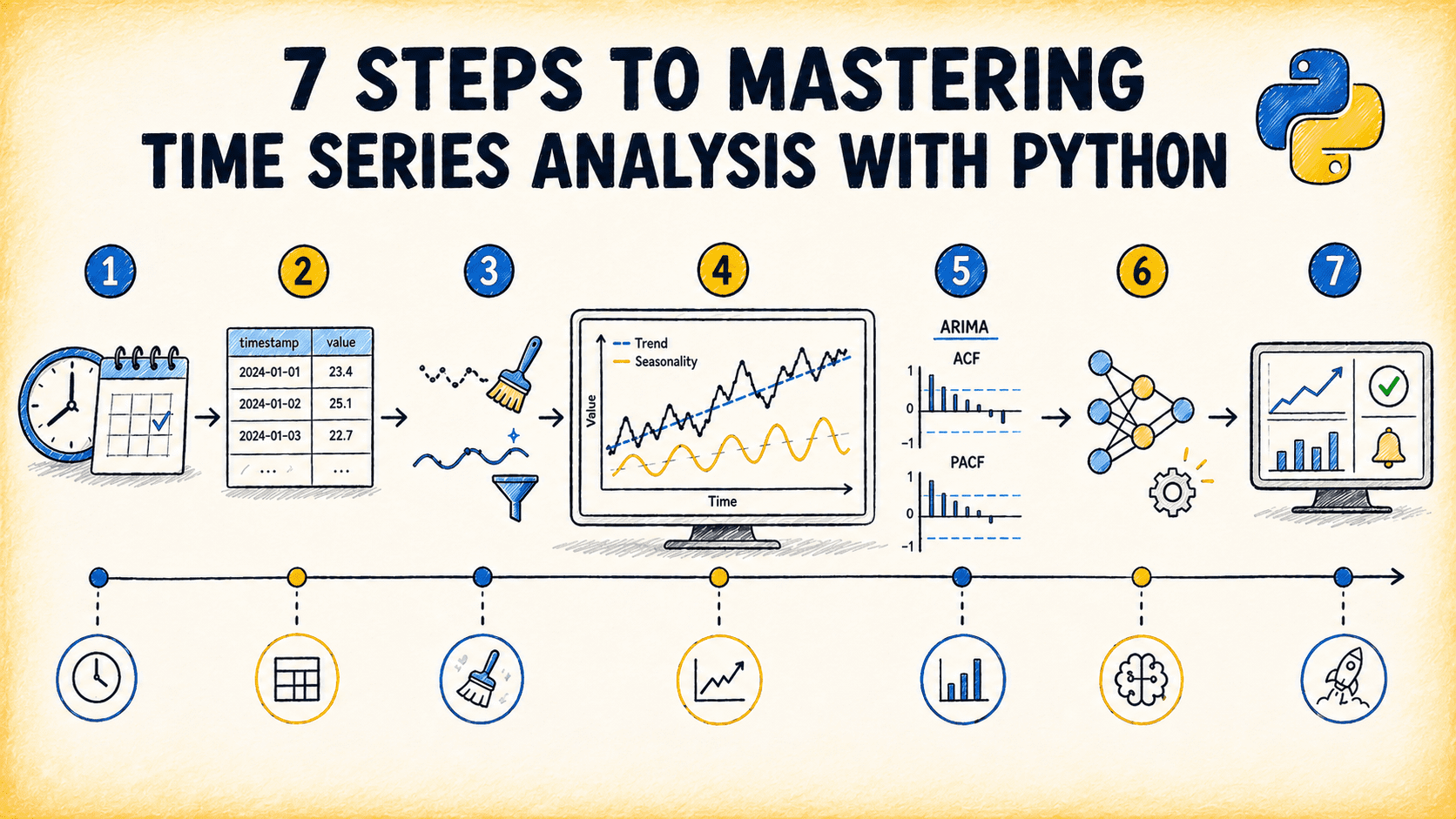
What makes time sequence distinct from normal knowledge science is that it calls for a unique psychological mannequin at each stage. Temporal ordering, autocorrelation, seasonality, and non-stationarity are structural properties that do not exist in tabular knowledge however outline the whole lot about how time sequence behave. The seven steps outlined on this article will enable you to study and develop into proficient in time sequence evaluation with Python.
# Step 1: Understanding What Makes Time Sequence Knowledge Totally different
To get began, it’s essential perceive the properties that make time sequence structurally completely different from tabular knowledge. Many practitioners skip this step, assuming normal machine studying information transfers straight. It does not, no less than not with out adjustment.
The three most essential structural properties are summarized under:
Property
What it means
Why it issues
Temporal dependence
Observations aren’t unbiased; what occurred yesterday correlates with right this moment
Commonplace machine studying issues assume row independence, so making use of it naively produces deceptive outcomes
Stationarity
Statistical properties stay fixed over time
Most classical fashions require stationarity; most real-world sequence lack it and want differencing or transformation
Seasonality and pattern
Common repeating patterns or seasonality mixed with long-run directional motion or pattern
Separating these from the irregular residual is commonly the core analytical problem
Useful resource: Rob Hyndman and George Athanasopoulos’s free on-line textbook Forecasting: Ideas and Observe (third ed.) is a complete reference. For those who’re serious about studying some critical time sequence evaluation, chances are you’ll wish to bookmark it earlier than continuing to any modeling step.
# Step 2: Mastering Time Sequence Knowledge Buildings in Python
Working with time sequence in Python means being snug with pandas’ time-aware knowledge buildings: DatetimeIndex, PeriodIndex, resampling, and rolling operations.
The excellence between DatetimeIndex and PeriodIndex issues greater than it first seems.
DatetimeIndex represents particular moments in time.
PeriodIndex represents spans of time.
Figuring out when to make use of every, easy methods to convert between them, and easy methods to parse, slice, and resample time-indexed knowledge saves important friction later, since most modeling libraries have particular format necessities of their very own.
Resampling and aggregation is the place many analysts make quiet, consequential errors. Downsampling from minute-level to hourly knowledge requires selecting the best aggregation perform, and getting it flawed corrupts the evaluation. Training resampling with a number of aggregation methods on the identical dataset till the logic is intuitive is time properly spent.
Rolling and increasing home windows — .rolling() and .increasing() — are the pandas primitives for lag options and cumulative statistics. Constructing rolling means, commonplace deviations, and lag offsets by hand earlier than counting on library abstractions is essential: understanding what these operations do on the index degree prevents a complete class of delicate knowledge leakage errors which are notoriously onerous to diagnose after the actual fact.
Useful resource: Work by the pandas Time Sequence and Date Performance information with an actual dataset earlier than continuing.
# Step 3: Studying to Clear and Put together Time Sequence Knowledge
Actual-world time sequence arrives with lacking timestamps, sensor dropouts, duplicate readings, and outliers. The cleansing selections made right here propagate by the whole lot downstream, and time sequence cleansing requires completely different strategies from tabular cleansing as a result of temporal ordering constrains each operation.
A lacking timestamp and a NaN at a gift timestamp are completely different issues. The previous requires reindexing to a canonical frequency grid earlier than imputation can find it. For NaN values, technique ought to match hole size and sign sort: time-based interpolation for brief gaps in steady indicators, ahead fill for step-function variables like tools states, and seasonal decomposition imputation for lengthy gaps in strongly seasonal sequence.
Outlier detection in time sequence calls for native somewhat than world considering:
World statistical thresholds can miss anomalies in non-stationary sequence.
Rolling Z-scores and IQR bounds over sliding home windows assist detect values uncommon inside their native neighborhood.
For multivariate sensor knowledge, Isolation Forest detects anomalies that will not seem in particular person channels however emerge throughout mixed options.
Frequency alignment deserves consideration when becoming a member of sequence recorded at completely different charges — hourly meter readings merged with day by day climate knowledge, as an illustration. The aggregation perform issues as a lot because the be part of itself, and documenting the downsampling logic is well worth the self-discipline, as a result of the selection impacts mannequin inputs in methods which are invisible within the merged output.
Useful resource: The sktime transformations documentation covers the commonest preprocessing transformations with useful examples.
# Step 4: Creating Instinct Via Exploratory Evaluation
You can’t mannequin what you have not understood, and understanding a time sequence requires structured exploratory evaluation earlier than any mannequin is match. Exploratory knowledge evaluation for time sequence goes properly past abstract statistics.
Decomposition ought to be step one in any critical evaluation. Utilizing statsmodels.tsa.seasonal.seasonal_decompose or the extra outlier-robust STL decomposition separates a sequence into pattern, seasonal, and residual elements, every of which rewards unbiased examination.
Is the pattern linear or nonlinear?
Is the seasonal amplitude secure, or does it shift over time?
Are the residuals roughly white noise, or do they comprise construction the decomposition missed?
Autocorrelation evaluation is the opposite important diagnostic. The autocorrelation perform (ACF) and partial autocorrelation perform (PACF) plots are the first instruments for understanding temporal dependence:
A slowly decaying ACF indicators non-stationarity.
Important spikes at lag 24 in hourly knowledge sign day by day seasonality.
PACF cutoffs counsel autoregressive (AR) order.
Studying these plots fluently is important for any classical modeling work.
Stationarity testing rounds out the exploratory workflow. The Augmented Dickey-Fuller (ADF) take a look at and Kwiatkowski–Phillips–Schmidt–Shin (KPSS) take a look at present statistical proof for or in opposition to stationarity, and operating each is worth it since they take a look at complementary hypotheses. The outcomes inform whether or not differencing or transformation is required earlier than modeling begins.
Useful resource: The statsmodels time sequence evaluation documentation paperwork the decomposition, ACF/PACF plotting, and stationarity testing capabilities you’ll use most often.
# Step 5: Constructing Classical Statistical Forecasting Fashions
Classical statistical fashions — ARIMA, Exponential Smoothing, and their extensions — ought to be the primary fashions you construct. They’re usually surprisingly aggressive with extra complicated approaches on clear, well-understood sequence, and so they pressure engagement with the construction of the information in ways in which machine studying fashions do not.
Exponential Smoothing (ETS) is the fitting place to begin. ETS fashions assign exponentially decaying weights to previous observations and canopy a variety of behaviors by additive and multiplicative elements for pattern and seasonality. Becoming a mannequin with statsmodels.tsa.holtwinters.ExponentialSmoothing and inspecting its elements provides instant instinct concerning the sequence’ construction.
ARIMA and SARIMA observe naturally. ARIMA fashions the autocorrelation construction of a stationary sequence by autoregressive and transferring common phrases; SARIMA extends this to deal with seasonal patterns.
Analysis self-discipline issues as a lot as mannequin alternative. Random cross-validation on time sequence produces optimistic and unreliable estimates; walk-forward validation — practice on the previous, predict the following window, advance the window — simulates how the mannequin would really carry out in manufacturing. TimeSeriesSplit from scikit-learn or sktime’s forecasting cross-validation utilities each implement this appropriately.
Useful resource: Forecasting: Ideas and Observe, Chapters 7–9 for ETS and ARIMA, and the statsmodels State House documentation for Python-specific implementation element.
# Step 6: Progressing to Machine Studying and Deep Studying Fashions
As soon as stable classical baselines exist, machine studying fashions permit richer function units, deal with complicated non-linearities, and scale to massive collections of sequence that may be impractical to mannequin individually.
Tree-based fashions corresponding to LightGBM and XGBoost produce sturdy forecasts when given well-engineered lag options, rolling statistics, and calendar variables. They deal with non-linearity and have interactions mechanically, however knowledge leakage is the central threat; lags have to be constructed strictly from previous values relative to the prediction timestamp. sktime’s make_reduction wraps scikit-learn regressors as forecasters safely and handles this bookkeeping appropriately.
World fashions develop into related when the issue includes a whole lot or 1000’s of associated time sequence — store-level gross sales, device-level sensors, regional power demand. Coaching a single world mannequin throughout all sequence usually outperforms particular person per-series fashions by sharing statistical power, and NeuralForecast helps this sample natively.
Deep studying architectures have the strongest observe information on benchmark datasets and deal with multi-seasonality, covariates, and long-horizon forecasting higher than classical fashions. NeuralForecast implements all of those with a constant API and correct temporal cross-validation help. The appropriate time to succeed in for deep studying is after easier fashions have plateaued, not earlier than.
Useful resource: Kaggle M5 Forecasting competitors notebooks are a very good place to begin, and the highest options cowl the complete pipeline from function engineering to ensembling on an actual retail forecasting drawback and are freely out there.
# Step 7: Deploying and Monitoring Forecasting Techniques
The operational challenges particular to time sequence are distinct from normal machine studying deployment.
Idea drift and distribution shift are inherent dangers somewhat than edge instances in time sequence, as a result of the sequence are non-stationary by nature. Monitoring forecast error metrics on a rolling foundation and organising automated alerts when error charges exceed thresholds is the baseline. Scheduled retraining pipelines aren’t non-compulsory in any manufacturing forecasting system.
Forecast storage and versioning require deliberate design. Manufacturing forecasting techniques generate predictions repeatedly, and storing forecasts alongside the actuals they predicted — somewhat than simply the ultimate mannequin outputs — makes it potential to compute retrospective accuracy at each horizon and perceive precisely the place the mannequin degrades over time.
Backtesting as a deployment gate is the self-discipline that separates experiments from production-ready techniques. Earlier than any mannequin goes reside, a rigorous backtest ought to simulate the complete deployment window utilizing solely knowledge that may have been out there at every step. A mannequin that appears good on a held-out take a look at set however fails a correct backtest shouldn’t be prepared.
Useful resource: Evidently AI’s mannequin monitoring information for machine studying monitoring together with knowledge and prediction drift detection.
# Wrapping Up
Time sequence evaluation rewards sequential studying greater than most knowledge science disciplines.
Step
Why it issues
Core properties of time sequence knowledge
With out understanding temporal dependence, stationarity, and seasonality, each subsequent choice rests on shaky floor
Pandas time-aware knowledge buildings
Right indexing, resampling, and window operations are stipulations for each evaluation and modeling job
Cleansing and preparation
Errors launched right here propagate silently by the whole pipeline; temporal ordering makes them tougher to catch than in tabular cleansing
Exploratory evaluation
Decomposition, autocorrelation plots, and stationarity checks reveal the construction that determines which fashions are applicable
Classical statistical fashions
Forces structural engagement with the information; usually aggressive with complicated approaches and at all times helpful as a baseline
Machine studying and deep studying fashions
Extends functionality to non-linear patterns, wealthy function units, and huge collections of sequence as soon as classical baselines are understood
Deployment and monitoring
A mannequin that can not be maintained in manufacturing shouldn’t be a completed product; time sequence techniques require domain-specific operational self-discipline
Basis fashions for time sequence — pre-trained on massive corpora of various sequence and fine-tuned for particular duties — are considerably altering how practitioners strategy forecasting. Constructing sturdy fundamentals in classical and machine learning-based approaches will definitely be helpful going ahead.
Bala Priya C is a developer and technical author from India. She likes working on the intersection of math, programming, knowledge science, and content material creation. Her areas of curiosity and experience embody DevOps, knowledge science, and pure language processing. She enjoys studying, writing, coding, and occasional! At present, she’s engaged on studying and sharing her information with the developer group by authoring tutorials, how-to guides, opinion items, and extra. Bala additionally creates participating useful resource overviews and coding tutorials.

